Finite Element Analysis (FEA) is indispensable for visualizing a structural response to a wide spectrum of loads and design options. FEA enables plotting a stress/strain field for complex geometries, which is not feasible to do by hand calculations. It appears that FEA services lose popularity in our industry. Here I share my thoughts why this happened, and conclude on how to improve the FEA practicality and to embed it into the plant asset management process. These tips are for FEA practitioners only.
Introduction – What is FEA at a glance?
Structural Mechanics force, displacement and stress calculations are well suitable for simple, idealized objects like beam frames (steel bridges, tower cranes, scaffolds etc.). Real structures usually have multiple ‘complications’ like joints and local stress raisers, and behave not as simple as the idealized analytical models. To combat the uncertainties of simplified calculations, structural designs always apply safety factors over the calculated parameters.
Material mechanics of continuum objects (truck trays, pressure vessels, rocket boosters and so on) usually become too cumbersome if attempted by hand calculations. FEA offered an essential relief to calculation engineers, by passing such tasks to computers. It became wide spread since 1990s, when powerful personal computers came. Over years, there was a variety of commercial FEA software, and even some free and open source options.
Tip 1 – FEA software choice
> Commercial FEA packages prices are grossly proportional to the number of features and their easiness of use. One very important point is the software capability for automatic AND manual meshing. Manual meshing is often necessary for making the FEA mesh do what you want, not the other way. Automated meshing is useful too. Good packages have both capabilities equipped with many options.
> Since all the FEA packages are bench-marked using a set of typical problems (developed by NAFEMS), their results precision is roughly the same – don’t expect the output precision to vary with price essentially. But check if the vendor provides bench-marking results.
> When choosing analysis modules in a FEA package, consider the physics you may need to model. For example, if you do structural design, then you will require at least linear statics and natural frequencies analysis as a minimum. Modelling electricity and fluid flow is something you may never need in this situation.
> Also be critical to specific engineering algorithms (fatigue analysis, pipe stress calculations, etc.) – these are rigidly bound to particular technical standards, not necessarily adequate ones in specific contexts.
> The major driver of the FEA output quality is the calculation engineer who drives the software – this is your most valuable asset, which takes years to educate ‘from scratch’ but is able to tackle unexpected problems, unlike computers.
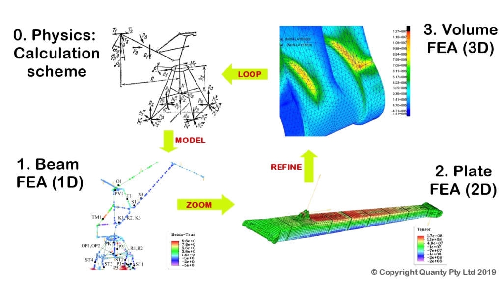
Under the bonnet, the FEA mathematical engine automates the calculation process by splitting a continuum object into many smaller elements connected at their nodes, together called the FEA mesh (see Fig. 1). The elements themselves can be spatially 1D, 2D or 3D. Computer assembles and calculates huge systems of equilibrium equations to estimate forces and displacements at each node. Next, it interpolates the displacements into stresses and strains of all the finite elements created by the user.
Why are they called ‘finite‘ – by their number, as opposed to practically infinite number of molecules within real steel crystals or other solid or fluid matter. A FEA model is therefore a coarse model of a continuum object. Typically, the more elements created – the better precision, but not always. Refining FEA model aims improving adequacy, and involves many aspects, not just the elements density per unit volume.
Tip 2 – Element type choice
Although the finite elements appear 1D, 2D, 3D (Fig. 1), all of them have more degrees of freedom (dof) – to store particular parameters sought, like beam curvature, hydro-static pressure, etc. As such:
1) Firstly we should select an element type with adequate dofs.
2) Secondly, quadrilateral and brick meshes converge to the reality better than triangles and tetrahedrons, as the latter are too stiff and sensitive to geometric distortions.
3) Thirdly, there is usually a choice of linear and quadratic elements. Edges of quadratic elements have additional nodes and can deform into curves, which improves the results precision. Edges of linear elements always remain straight and may serve as false stress raisers. Ultimately, a same precision of results may require roughly 10 to 100 times finer mesh made of linear tetrahedrons compared to quadratic bricks. This is a major source of overlooked issues from automatic tetra-meshers use.
A good software manual clearly details such nuances.
FEA modeling is applicable to a variety of physics science branches. For example, some advanced NDT companies can model even ultrasonic beam propagation and reflection within a specific part – to establish a baseline picture: what they see on the screen and what does it mean. Here we will only focus on the common structural stress/strength analysis applications.
Trick of the tricks – Know you physics!
An absolutely utmost importance in FEA application is modeling the right mechanical phenomenon. A practitioner must understand the role of the model in the decision making process – What are we looking for and why? This sounds quite obvious, but pitfalls are numerous:
Question 1: A process pipe of a critical risk operates in a cyclic temperature service. The problem is the fatigue life prediction – what is the safe operational life?
Answer 1: The designers completed a pipe stress analysis before. Let’s use their figures. WRONG: Pipe stress software employs 1D elements (with no circumference coordinate), while our concern stresses are essentially localized (Fig. 2). Also, design case thermal stresses might not match the operational case. Look deeper.
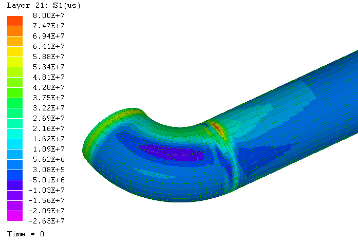
Answer 2: Let’s measure the pipe temperature in-situ and apply it to the plate model (Fig 2). NOT CONSERVATIVE: There might be other loads (like pressure and vibration) which will drastically reduce the fatigue life. Besides of this, we will need to model the whole piping circuit, with many temperatures measured and applied. How about pipe supports – can we model their reactions confidently?…
Tip 3 – Balance Complexity and Adequacy
Is a more complex model more comprehensive? I thought so in the very beginning: the more parameters we include in the model – the better will be the result (for example – the mentioned pipe supports modeling). In fact, the more parameters our model requires – the more uncertain values we feed in the model, and then – assume being a true output.
An example uncertain parameter can be a structural damping in a harmonic (dynamic) response FEA. As many joints and contacts the structure has – so many damping coefficients we need to apply in the model. What is our confidence in these values? There is a good way around though – in-situ hammer test: bump that structure slightly and measure the attenuation of oscillation. The measured attenuation rate can be converted into the actual damping coefficient of the real object we bumped.
As a rule of thumb, in-situ measurements greatly improve FEA modelling simplicity and certainty. Design case FEA models can be complex, but their inputs and outputs are commonly in doubt.
Getting back to the question, Answer 3: Let’s measure stresses in-situ (using strain gauging) and calibrate the plate FEA model to mimic them. GOOD: this is a comprehensive solution with a good chance of adequate prediction, providing that we select a relevant weld material fatigue curve. Our stress hot spot in Fig. 2 is located at a butt weld seam indeed.
This is now a point where practical integrity engineering should contribute:
Answer 4: Is there anything we have missed? RIGHT, there might be a crack of a detectable size already present. We need to perform a crack detection survey as a matter of precaution. And if we have actually detected a crack – this is not a fatigue theory anymore, but a fracture mechanics problem, refer to Fitness-For-Service standards.
The number of issues above is worrying, showing the challenges of practical integrity assessments, as opposed to basic design. FEA aided design is relatively straight-forward, as all load cases and fitness criteria are defined in the design standards (refer this post for design vs assessment comparison). But still, is that all? All good? Next sections will show few fundamental issues, associated with any structural FEA application.
Trick 1 – Beam model of the whole
The beam theory provides precise analytical solutions, only available for simple problems (cantilever beam in bending, crane joints reaction forces, see Fig. 1, and similar). And obviously, this applies to beam-like objects only.
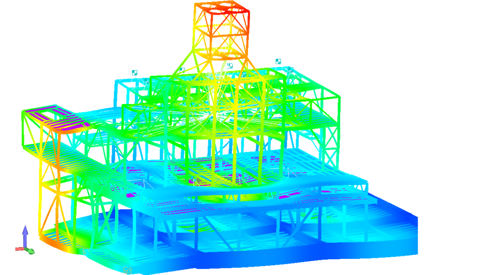
If we run a validation case for say, a bridge span sagging, using manual calculations versus FEA – the results must be the same. Because the problem is simple enough for a hand calculation. In turn, this means that a beam FEA model has no better precision than the beam theory itself. Still, FEA has few universal benefits, regardless of the model/element type:
- Fast calculation of complex geometries (Fig. 3)
- Easiness of changing and re-evaluating various load cases and values
Tip 4 – Linear problems versus Design Cases.
If our system’s response is linear elastic (no yielding or mechanical contacts), then a proportional increase of the load will drive same increase in the displacements and stresses. A force increase of X% will drive the stress increase by same X%. Use coefficients.
Issues occur when several loads are applied to the model and varied disproportionally among the load cases. Say Force A by X% and force B by Y%, and so on – the stress/strain implications become not so obvious as above. This is where FEA automates the re-valuation process very well. Just change the loads and re-calculate.
There is one serious shortcoming of the beam elements though: inability to model local stresses (see red spot in Fig. 2). Beam FEA (Fig. 3) ‘knows nothing’ about stress raisers present in our structures. Beams are beams, they can bend and twist, but only as a whole. Whatever happens at local geometry discontinuities (gussets, attachments, elbows, weld profiles themselves) – we can’t evaluate that using just beams and rods.
Tip 5 – Results are limited to the modeled behavior
Why do engineers believe they can analyze pipe stresses using beam FEA based software? Because they were told the analysis is done to the relevant standard. But that is a DESIGN standard. We have analyzed the difference of design and assessment approaches here.
Displacement analysis – Yes. Nominal stress analysis – Yes. Local stress analysis using beams – NO. Beam elements simply don’t have that degree of freedom (circumferential coordinate) where the complex stress field develops (Fig. 2). Sadly enough, the damage (either plastic flow or cracking) will progress where the stresses are the highest. The beam element abstraction is not suitable for detailed stress modeling, unless stress concentration factors are introduced manually, but again – what is our confidence in them?
Trick 2 – Structural Zoom
Whenever a structure of concern is made of beam-like (slender) members, the analysis sequence and cost can be well optimized as follows (see Fig. 1):
- Coarse analyze the whole structure using beams
- Tabulate the reaction forces and moments output
- Model just fragments of highest stresses using plates
- Load this fragment with the reaction forces from step 2
- Analyze plate models for local stresses at a sufficient resolution
This ‘structural zoom‘ approach is very useful for welded structures. A piping circuit is a welded structure too. We can can also do a zoom from 2D (plate) to 3D (volume).
Some objects require plate models from the very beginning, as they aren’t slender beams at all (vessel shells, tank roofs, engine brackets and so on). Some objects are nothing but 3D bodies and plate modeling of them makes no sense (these are various castings and machined parts: pump manifolds, turbo-fan engine blades, etc.). But the idea of zooming should be kept in mind anyway. IN this way, we can limit the most complex modeling to the concern objects/areas only, in order to save time.
Trick 3. What stress components are we after?
Again, know your physics. There is a variety of stress components available for plotting. The most popular are the Maximum Principal and the VonMises equivalent stress. And surely, you will read different values from them. A good question is almost a good answer: What are you going to compare?
Example 1. Fig. 2 pipe operates at above ambient temperature and is overloaded statically (say, a pressure vessel may hang on it for a while). That is a material yielding problem, and the VonMises stress will be a good value to compare with the material yield strength.
Example 2. Same pipe and load case, but during a winter time shutdown, in Alaska. Here we need to look at the material toughness, and the Ultimate Tensile Strength (UTS) reduction due to the ‘cold embrittlement‘ effect. At low temperatures, UTS can become very low, hence a brittle fracture is credible and the Max Principal (maximum tensile) stress should be checked with the UTS.
Example 3. Same pipe in an ambient temperature, but the vessel becomes hanging on the pipe suddenly (on a support failure). Aha, dynamics! As a first crude pass, this would require comparing the dynamic Max Principal stress with the UTS too. However, the weld at elbow could have triggered small cracks nearby (due to material shrinkage on cooling). If so, it becomes a dynamic fracture mechanics problem.
Tip 6 – Ductile failures versus Brittle failures
Plasticity requires warmth and some amount of time to develop. As it becomes colder – the inter-crystalline bonds weaken, and the structure prefers breaking rather than yielding (that is the apparent UTS reduction).
Similarly, if we apply the load too suddenly, the material simply has not enough time to yield, and does fracture at the hot spot. A brittle fracture is in fact a crack propagation subject.
All kinds of fatigue are intermediate phenomena: there is a local plasticity and material tearing at a crack tip simultaneously. The proportion depends on the above factors: temperature and strain rate. The outcomes depend on the number and amplitude of the load cycles, as we know from the phenomenological fatigue theory.
Metal grain size also influences the tendency for brittle fracture. The smaller the grain – the more barriers are on the crack’s way. Welding produces larger grains and generates residual stresses.
Books on mechanical behavior of materials well detail this topic.
Overlooking the above nuances can render an inadequate selection of the stress components and their allowable values: The 1st major issue prominent in the FEA practice: the problem description can be narrowed to what FEA can do, while the real problem needs more than FEA does, in order to be solved.
The 2nd major issue of FEA applications is the stress convergence problem, which is handy to observe from the above pictures:
Firstly, look at the crane boom (pos. 2 in Fig 1) – its top shelf is consistently red with a +/- 25 MPa variation. The stress gradient is smooth and not localized. This suggests that the stresses converged well. For an added security we may try using smaller elements, then running a sensitivity study.
Secondly, observe the local hot spot (red) in the Fig 2. It has a sharp gradient. Hence, we need to refine mesh to have at least few elements within the gradient zone. Some good news here – this stress field will gradually converge to a certain value as the size element decreases (simply because there are no geometric stress risers modeled in Fig. 2). But in fact – there are stress raisers – the non-modeled weld profile. Let’s keep going…
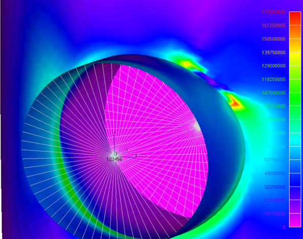
Thirdly, the Fig. 4 shows a crack (a free surface within the material), FEA modeled as a linear elastic material problem. This problem is singular – the stress will tend to infinity, and will never converge. This is because the material plastic flow is not included in such a model. Notably, a similar non-convergence can occur with other sharp stress raisers (triangular gussets, perfect 90 degrees joints with no weld radii, and others). In reality – there won’t be an immediate rupture, but a plastic zone will form by the yielded material. Whether this is critical or not? We can reply via using a ‘flow stress‘ limit for ductile problems, while for brittle failure and cyclic loads problems we can evaluate Stress Intensity Factors . Fitness For Service (FFS) standards merge these failure criteria and evaluate failure potentials as a combination of ductile and brittle options discussed above.
Tricking FEA outputs
What exactly we mean under the term ‘stress‘ depends on the calculation goal (see Fig. 5):
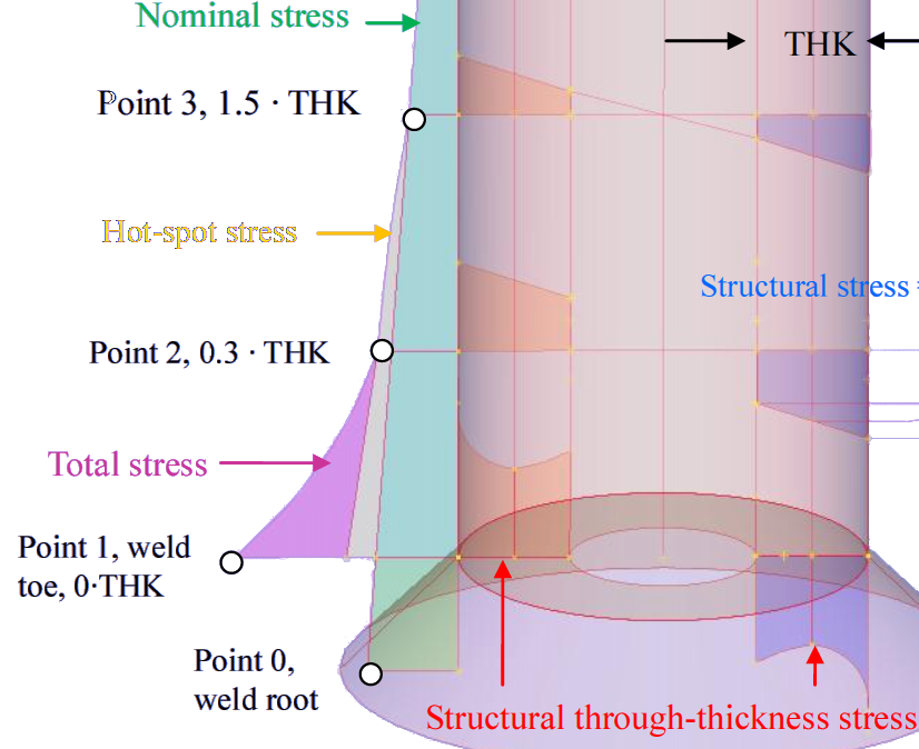
- Nominal is a gross section stress (green), often found from hand calculations
- Local is a FEA stress extrapolation to the stress raiser (yellow)
- Peak is an elevated stress at a notch (red), sensitive to the FEA convergence issue
Each of the three options produces a different value for a selected stress component. Luckily, there are criteria to identify the correct option:
Trick 4.
We don’t need to know the crack tip stresses (Fig. 4) as the fracture mechanics Stress Intensity Factors (SIF) account for them implicitly.
We need to know the local stress (yellow, Fig. 5) along the crack path.
Trick 5.
We don’t need to know the peak stress at the elbow weld toe (Fig. 2) as relevant fatigue testing data already includes this stress raiser effect.
We need to know the local stress (yellow, Fig. 3) made by our particular loading of this very joint, for the fatigue curve input.
Trick 6.
We don’t need to know a peak or local stress for a comparison with UTS or with yield strength, as material strength figures are standardized, tested and reported as engineering stresses in a nominal section of an intact specimen.
We need to know nominal stresses (green, Fig. 5) for material strength comparisons, which is the dominant case of design calculations.
FEA can enable all the above outputs, while their purpose must be kept in mind, for example:
Looking at the Fig. 2, we can draw conclusions on whether a plastic joint will form (providing that the red hot spot stress converged), or a brittle fracture may/may not occur, depending on our ductile-brittle conclusion. This applies to the local (red) section. Nominal stresses in the gross (green) section suggest whether we may/may not have a problem, and what is the safety factor. This is a design case application of FEA.
Regarding the crack tip red peak in Fig. 4 – it must not be compared with standard strength figures, neither with any other figures as this output is singular and non-converging. Instead, the local stress field along the crack path (green gradient in Fig. 5) goes for use in a fracture mechanics based apparatus, such as from FFS standards. This is an assessment/troubleshooting application of FEA.
The following applicability generalizations apply:
- Nominal stresses (green in Fig. 5, either from FEA or not) are for standard design checks and safety factors evaluation. Local and peak FEA stresses can be over-conservative for this goal.
- Local stresses (yellow, Fig. 5) are for phenomenological damage models (plastic collapse and fracture assessments, FFS). Such models are useful for integrity assessments of actual objects in true operational conditions, as opposed to factored designs
- Peak stresses (red in Fig. 5) only make sense to compare with peak strengths (true stress and strain), which are not standard. This is because actual failures occur as a result of material imperfections growing in service (cracks, corrosion, creep, etc.). Phenomenological (best fit) models help well with these issues. These models demand either nominal or local stresses, depending on whether the testing data reflects a particular geometry (fatigue of weld details) or a particular material (such as fracture toughness or creep properties).
Tip 7 – Minimum Design Strengths
An additional source of confusion is the ‘specified minimum strength’ from design standards. Those ‘specified’ figures are either yield strength or UTS, already generously factored for safety (3.0 to 4.0 times in pressure design). Naturally, comparing the FEA stress hot spots with these figures triggers alarms all over. For example, a code specified minimum yield strength (SMYS) of a steel can easily go down to 120 MPa, and the Fig. 4 green stress ring would have failed the checks. This is a false alarm, as we should first ‘restore’ the material property – remove factor of say 3.5 to get 420 MPa, then – re-evaluate the safety factor, that is 420MPa/130MPa = 3.2, and finally – decide on whether we accept that or not in view of the relevant damage physics, such as material fatigue.
As a result, not the FEA itself, but the FEA mis-applications triggered the client side reduced confidence and interest over the recent years. One aspect of improvement is avoiding the mistakes mentioned in this article. Another aspect is understanding the FEA as a tool within the assessment and decision making loop. That is: FEA output must fit the decision making criteria (e.g. standardized methodologies) of a particular phenomenon assessment (like crack propagation, cold rupture, creep), whatever is relevant to the actual operation of a particular object (know your physics).
Few more examples of FEA application spectrum at industrial plants:
- static stress/strength analysis in designs and of flawed equipment, meaning identifying safety factors and predicting remnant lives
- dynamics: natural frequencies, harmonic and impact spectra response, meaning vibration and shock analysis and controls evaluation
- input data for fatigue/fracture/environmental cracking problems, meaning setting risk controls for cracking damage types
- thermal and thermal stress analysis, electric fields modeling if required
- computational fluid dynamics and variations, meaning fluid flow and dispersion analysis, fluid pulsation, water hammer modeling, etc.
Way forward
FEA is an indispensable instrument for integrity assessments and for equipment design. What happened unfortunately – clients refrain from paying FEA added costs for achieving same (deterministic) outcomes readily available from equipment design documentation. The benefit of equipment integrity assurance and optimization using FEA is not effectively realized in industries other than ‘hi-tech’ ones (nuclear, aircraft, medical prosthesis and rocket building). Nevertheless, there is a huge potential of life-cycle cost savings yet hidden for infrastructure and resource sectors.
The modern asset management concept aims providing a cost/benefit optimization framework transparent for all levels of an organization. The major drivers are therefore risk levels and comparative costs. The concept is entirely applicable to integrity analysis level decisions. It is often said that the cost of fixing error at a design stage is an order of magnitude less that the cost of fixing it when the design operates already. Same applies to plant integrity management in operation: it is an order of magnitude cheaper to analyze the problem and mitigate it at a right time, rather than waiting until an actual failure occurs and triggers vast financial (and often – safety and environmental) consequences. Decisions must be risk driven.
Therefore, FEA can be embedded in the asset management process as a viable and holistic analysis tool relevant to equipment integrity risk control. Organizations with asset management systems implemented to ISO 55001 should be automatically conductive organizations for such an perspective. And there is a clear driver to initiate this evolutionary change: the typical asset management goal (get most good from the equipment and minimize any bad happenings) is well facilitated by a risk based FEA implementation for critical assets (those with severe implications of failures).
P.S. This article aimed a big picture of FEA capabilities, application pitfalls and of asset value adding perspectives. Technical rigor was sacrificed in some extent to make the explanation of nuances ultimately simple and widely perceivable. The entertaining concept of ‘trickonomy’ was applied to simulate an adventure and gaming atmosphere. The topic is nevertheless very serious regarding knowledge demands and decision making consequences. The reader should consult with more formal literature, relevant standards, and/or with us, prior to making any such decisions. I hope you liked this material compiled from my 10 years exposure to FEA and 10 years exposure to integrity risk assessments. Either way, you are very welcome to comment this post or leave us a direct message.